Trane vs. TAS – Desiccant Wheel Simulation Comparison

Trane vs. TAS – Desiccant Wheel Simulation Comparison

This document shows how TAS Systems can comply with the rated performance of desiccant-based dehumidification systems, as documented by Trane in the Engineering Newsletter volume 34-4. Each different arrangement of desiccant wheel has been modelled in TAS Systems to match the performance of the Trane examples shown via psychometric charts. These have been closely reproduced in TAS.

The performance characteristics have been taken directly from Trane and can be found in the following location:

http://www.trane.com/cps/uploads/userfiles/educationalresources/admapn016en_0905.pdf

1.0 – Wheel Upstream of Cooling Coil

1.1 – Model Comparison

Traditional desiccant dehumidification wheels in a parallel arrangement rotate between two air streams. The regeneration air stream (RG) may be a building exhaust that is used exclusively to reactivate the desiccant. The RG is heated in order to raise the dry bulb temperature and, in turn, lower the relative humidity. This results in water vapour being transferred from the OA stream to the RG’ stream. Although the desiccant wheel removes latent heat (moisture) from the process air stream, sensible heat is added. A cooling coil is often required downstream of the desiccant to cool the air to a practical and usable temperature.

Figure 1 – Trane Wheel upstream of cooling coil model
Figure 2 – TAS Wheel upstream of cooling coil model

1.2 – Psychrometric Chart Comparison

Figure 3 – Trane Psychrometric chart for wheel upstream of cooling
Figure 4 – TAS Psychrometric chart for wheel upstream of cooling

1.3 – Results Table Comparison


 Trane temp (F)TAS temp (F)Trane Rel hum (%)TAS rel hum (%)
RG87.087.069.0069.00
RG’250.0250.01.47
RG”135.0134.336.79
OA87.087.069.0069.00
OA’145.0146.84.19
CA77.077.049.0049.13

Figure 5 – Results table for wheel upstream of cooling coil

2.0 – Wheel Downstream of Cooling Coil

Generally speaking, most desiccants adsorb more water vapour as the relative humidity of the process air rises. Desiccants also adsorb more water as the dry bulb temperature of the process air falls. During the cooling season, the coldest part of the system is that which is directly downstream of the cooling coil. It is for this reason that it would be desirable to place the desiccant wheel downstream of the cooling coil, rather than upstream, as in the previous example.
This wheel downstream configuration is mainly used in dedicated outdoor air applications. Relative to the wheel upstream arrangement as used previously, the same dehumidification can be achieved to the same dew point but less or no recooling is required.

2.1 – Model Comparison

Figure 6 – Trane wheel downstream of cooling coil model
Figure 7 – TAS Wheel downstream of cooling coil model

2.2 – Psychrometric Chart Comparison

Figure 8 – Trane Psychrometric chart for wheel downstream of cooling coil
Figure 9 – TAS Psychrometric chart for wheel downstream of cooling coil

2.3 – Results Table Comparison


 Trane Temp (F)TAS Temp (F)Trane Rel Hum (%)TAS Rel Hum (%)
RG1061064140.98
RG’114.0114.032.0032.52
RG”106.0106.241.0042.60
CA62.062.096.0096.00
CA’77.076.849.0048.81

Figure 10 – Results table for wheel downstream of cooling

3.0 – Series Desiccant Wheel in a Mixed Air Application

Series regeneration in a desiccant system places the regeneration side of the wheel upstream of the cooling coil and the process side downstream of the coil. Moisture is adsorbed from the process air downstream of the cooling coil and is placed back upstream of the coil. This negates the need for a separate regeneration air stream.

Air leaving the process side of a series desiccant wheel is cooler that the space, making this kind of system good for use in a mixed air stream, with one unit being able to cool and dehumidify the air.

3.1 – Model Comparison

Figure 11 – Trane series desiccant wheel (series regeneration) in a mixed air system model
Figure 12 – TAS series desiccant wheel (series regeneration) in a mixed air system model

3.2 – Psychrometric Chart Comparison

N.B in figure 13, the relevant points for the mixed air flow system are; MA, MA’, CA, SA

Figure 13 – Trane Psychrometric chart for series desiccant wheel in a mixed air application
Figure 14 – TAS Psychrometric chart for series desiccant wheel in a mixed air application

3.3 – Results Table Comparison

 Trane Temp (F)TAS Temp (F)Trane Rel Hum (%)TAS Rel Hum (%)
MA80.080.043.0043.00
MA’74.074.164.0058.02
CA51.051.092.0092.00
SA56.056.962.0063.70

Figure 15 – Results table for wheel in a mixed air application

Closing statement about differing temperature change (5F vs 6F)

Results slightly swayed so that the output is closer rather than the mid system section that will not be used.

4.0 – Series Desiccant Wheel in a Dedicated Outdoor Application

A series desiccant wheel can also be used in a dedicated outdoor application because the wheel adds little sensible heat to the process air. This means that the dry bulb temperature of the process air is cool enough to use. This application can be compared to the ‘Wheel downstream of cooling coil’ arrangement that was considered earlier. In the same conditions the series wheel delivers air at the same dryness but at a cooler temperature than the downstream wheel.

4.1 – Model Comparison

Refer to 3.1 – System layouts used are the same

4.2 – Psychrometric Chart Comparison

Figure 16 – Trane Psychrometric chart for series desiccant wheel in dedicated outdoor application
Figure 17 – TAS Psychrometric chart for series desiccant wheel in dedicated outdoor application

4.3 – Results Table Comparison


 Trane Temp (F)TAS Temp (F)Trane Rel Hum (%)TAS Rel Hum (%)
OA87.087.069.0069.00
OA’81.080.987.0085.92
CA58.058.098.0098.99
CA’64.064.177.0076.33

Figure 18 – Results table for a wheel in an outdoor air application

Use of Single Zone VAV Systems

Use of Single Zone VAV Systems

1.0 - Introduction

The purpose of this document is to outline some of the ways TAS Systems has the ability to model single zone VAV systems and their performance characteristics with particular reference to the Trane Engineering newsletter Volume 42-2, entitled ‘Understanding Single-Zone VAV Systems’. The newsletter can be found at the link listed below. Trane Engineering Newsletter Volume 42-2 A single zone constant volume system traditionally uses a temperature sensor in the designated zone in order to vary the cooling and heating capacity, whilst the fan supplies a constant quantity of air. A single zone VAV system, on the other hand, uses the temperature sensor to vary the airflow delivered by the supply fan as well as the heating and cooling capacity in order to maintain the supply air temperature at a set point. Single Zone VAV systems for the most part have been used for large, densely occupied zones that have varying cooling loads. These can include lecture halls, sports halls, and large meeting rooms. As a greater concern for energy consumption develops, single zone VAV is now being increasingly used in smaller zones such as offices, retail stores and classrooms, to take advantage of the energy saving capabilities that can be associated with single zone VAV (SZVAV) systems.

2.0 - Relevant ASHRAE Requirements

Requirements of the ASHRAE Standard 90.1 has certain specifications that single zone VAV systems must comply to. The requirements vary depending on whether cooling coils or direct expansion cooling is utilised. These are listed below;

  1. Air-handling and fan-coil units with chilled-water cooling coils and supply fans with motors greater than or equal to 5 hp shall have their supply fans controlled by two-speed motors or variable-speed drives. At cooling demands less than or equal to 50%, the supply fan controls shall be able to reduce the airflow to no greater than the larger of the following:
    • One-half of the full fan speed, or
    • The volume of outdoor air required to meet the ventilation requirements of Standard 62.1.
  2. Effective January 1, 2012, all air conditioning equipment and air-handling units with direct expansion cooling and a cooling capacity at AHRI conditions greater than or equal to 110,000 Btu/h that serve single zones shall have their supply fans controlled by two-speed motors or variable-speed drives. At cooling demands less than or equal to 50%, the supply fan controls shall be able to reduce the airflow to no greater than the larger of the following:
    • Two-thirds of the full fan speed, or
    • The volume of outdoor air required to meet the ventilation requirements of Standard 62.1.

3.0 - How can TAS Meet These Requirements?

3.1 – First to model the system

The basic model for a single zone VAV system in TAS is shown in figure 1. This uses a heating and cooling coil to vary the temperature of the supplied air with an optimiser used to control the mixing of the outside air and the return air coming back through the system. The heating and cooling coils are controlled by the thermostat in the zone as well as reading the temperature leaving the fan in relation to heating and cooling setpoints.

Figure 2 shows a very similar system that uses direct expansion for the heating and cooling in place of a heating and cooling coil. 

3.1.1 – Optimiser (economiser) in place of dampers

The Trane Engineering newsletter speaks of the implementation of dampers to control airflow. Although TAS has the ability to implement and control the dampers, in this single zone VAV model, TAS has a simpler method of control. An optimiser can be set up so that it will supply as much air as is necessary to the zone from mixing recirculated air and fresh air, whilst ensuring that the minimum fresh air for the zone is met. This is a simpler method for the user to control the ventilation in TAS systems. A complex control circuit would need to be made if dampers were to be used. Figure 6 shows the use of the optimiser in place of the mixing box the Trance Engineering newsletter references. This optimiser is used in both figures 3 and 4. 

3.2 – Minimum flow fan speed – ASHRAE

TAS Systems has the ability to model both cooling and heating coils as well as direct expansion as a means of cooling and heating. The ASHRAE requirements are easily met by inputting some parameters into the software. The requirement A is met in TAS by adjusting the fan properties in a model that uses a cooling coil to generate the cooling capacity. The fan is sized so that it can meet the maximum flow at any one time, whilst the minimum flow source is set to be 0.5x the design flow source. The other requirement, regarding outdoor air ventilation standards is set to ‘all attached zones fresh air’, which is specified in the occupancy conditions of the zone in TAS. In this case there is only one zone attached and the fresh air requirements never exceed one half of the full fan speed. The inputs for this are illustrated in figure 4. Requirement B is similarly implemented in TAS on a model that uses direct expansion to cool and heat the attached zone. The minimum flow on the fan is required to be two thirds that of the full fan speed. This is done by setting the minimum design flow fraction to be 0.6667. Similarly to the previous example, in this case the fresh air requirements will never exceed the two thirds of the full fan speed, meaning that the minimum fan flow rate will be 102.8 l/s during operating hours. The inputs for this are illustrated in figure 5. 

3.3 – CO2-based demand-controlled ventilation

The Trane document outlines how single zone VAV systems are often used for zones that experience largely varying populations. As the population increases, this means the occupants produce more CO2. These zones can be controlled using a carbon dioxide sensor to maintain a comfortable working area with sufficient fresh air to breathe. A carbon dioxide sensor can be used to control an increase in the air flow when the CO2 levels exceed a specified level. This method is implemented into TAS Systems as shown in figure 6. The values for desired CO2 levels can be edited with ease. The blue cross marks the controller monitoring the carbon dioxide, which is located in the exit air stream from the zone being controlled. Another method of controlling this would be to use a damper at the outside air inlet, controlling its opening by a similar CO2 sensor. 

4.0 – Types of Fan control

There are varying methods of controlling single zone VAV systems including how and when they cool or heat and at what flow the supply fan will operate. The three main types of fan control to be looked at are:

  • Constant-speed fan
  • Two-speed fan control
  • Variable-speed fan control

Each method of control is modelled separately in TAS Systems. The constant-speed fan model simply has no controller connected to the fan, meaning that it runs at the sized load whenever the system is in operation. Due to TAS using an hourly sampling system the two-speed fan control cannot be modelled as it would in a real system. This is because it would require instantaneous adjustment and calculation with relation to the flow rate. For this reason, the two-speed fan is modelled the same as the variable speed fan. This can be done because, if the fan speed is say 0.5x the full capacity, this means that a two speed fan will have been doing the same overall work but the speed output TAS gives can be interpreted as a proportion between the two fan speeds that it operates at. The two-speed fan and the variable speed fan are distinguished in their energy consumptions by their differing part load characteristics. Load in a variable speed fan is not directly proportional the power. With a two-speed fan however, it can be assumed that each fan is operating at peak load, allowing it to be modelled by a directly proportional part load characteristic. The variable speed fan differs from this, in that under low loads it uses less power, meaning that it saves on power usage relative to the other two fan control methods. The part-load characteristics are shown below in figure 7. 

5.0 – Energy Savings Associated with SZVAV

As stated and shown in the Trane engineering newsletter, energy savings can be expected by the utilisation of two-speed and variable-speed fans over the dated method of supplying the attached zone with a constant supply of air. Trane supplies results for three different types of fan system, showing how much energy could be saved with the implementation of the two improved fan control methods. Below, figure 8 shows energy consumptions for a classroom in three different locations in America as given by Trane. Figure 9 shows energy savings as found by a simulation in TAS Systems with weather data taken for Sydney, Australia. It can be seen that from the two graphs energy savings are similar for the two-speed and variable-speed fans relative to the constant speed set up. The reasons for the different savings in the Trane and TAS models can be attributed to the varying building size, building layout, climate and operating hours that heavily influence the energy saved. 

6.0 – Improved Part-Load Dehumidification with SZVAV

There is a noticeable difference in the performance of a constant volume system relative to a single zone VAV. The latter improves dehumidification performance at part load conditions. Below in figures 10 and 11, it can be shown graphically via a Trane example and an example done using TAS systems. At part load, the constant speed fan supplies a constant volume of air to the zone. As the sensible cooling load in the zone decreases, the compressor cycles on and off, resulting in warmer air being delivered to the zone. This results in a warmer average coil temperature, meaning that the warmer air has not been dehumidified as much as if it had been cooled more by the single zone VAV system. The single zone VAV system, instead of switching off the compressor, reduces the supply airflow whilst still cooling to the same temperature. This allows more moisture to be removed from the air, giving better dehumidification to the zone. Although more cooling load is applied, more energy is saved from reducing the fan energy. The dehumidification performance values from Trane and TAS Systems are given in Tables 1 and 2 respectively. 

Constant Speed FanVariable Speed Fan
84oF DBT  
Zone Humidity, %RH74%63%
Cooling Loads, tons0.2160.345
Fan Airflow, cfm482291

Dehumidifying With Constant Volume Systems

Introduction

The purpose of this document is to look at dehumidification performances in a constant volume system, with specific reference to the Trane engineering newsletter ‘It may take more than you think to dehumidify with constant-volume systems’ volume 29-4. These performances will be simulated in TAS Systems to show the software’s capability of modelling such systems. The newsletter referenced looks at how constant volume systems often provide difficulties in dehumidification of zones and how different strategies can get the best performance out of the system. It can be found at the link below.
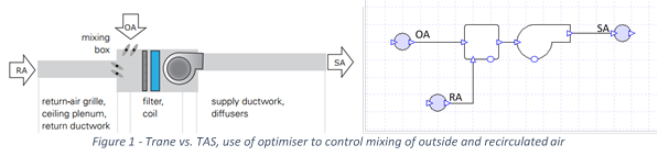
A basic constant volume system will be made up of an air handler serving a single thermal zone. This provides the zone with a mixture of outside and recirculated air that has been adjusted to a required temperature. This temperature is decided by a thermostat within the zone that compares the zone temperature to the set point. The supply air temperature is changed until the sensible capacity of the coil is sufficient to cool the zone to the set point.
Often designers of these systems will size the cooling coils based on the peak sensible load. This load is when it is hottest outside, i.e. the hottest day of the year. However, the latent load on the cooling coil peaks when the outside dew point is the highest. This can mean, in some cases, that the air handler may not have enough capacity to cool the zone, and in part sensible-load conditions it will neglect to reduce the humidity of the zone sufficiently.
At peak sensible cooling, the coil cools the air to the required temperature whilst indirectly removing the latent heat from the air. At part-load conditions this becomes a problem. In order to reduce the cooling the temperature of the cooling coil is raised. This means that there will be less condensate produced over the coil and the humidity of the zone is often too high.
Each of the system arrangements, will be analysed at peak sensible load as well as peak latent load. This will show how at peak sensible load, the cooling coil temperature is increased slightly so that the sensible loads are met. This then means that less latent cooling is done, often resulting in an unsatisfactory humidity level in the zone.
It is worth noting that the results from Trane and TAS are somewhat different. This can be subject to different building models and sizes as well as operation gains and climate. The TAS example is taken to be a small classroom in Australia. This is hotter than the example that Trane uses in America. Also the Trane design condition for sensible load there is no present latent load. This means that, for example, the supply-air tempering model operates as a simple CV system. In the TAS climate however, the system is designed to remove this humidity from the system, hence the higher cooling loads of the systems. The latent load is also higher at the latent design for the TAS simulation than in the Trane data used.

Basic CV System


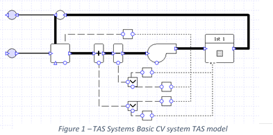
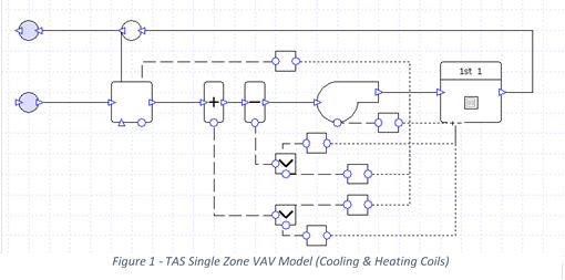
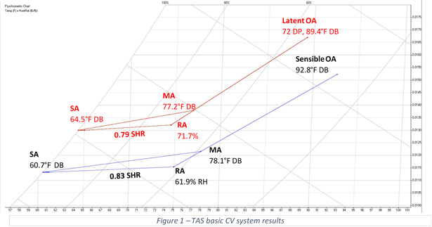
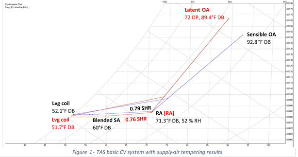
The basic constant volume system used is a simple one that was modelled in TAS systems. Any dehumidification in this system is a by-product of the sensible cooling done by the cooling coil to reduce the air temperature of the zone. Figure 1 below shows the model configuration.
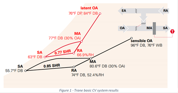
The results from Trane as well as those from the TAS simulation tell a similar story. The dehumidification at the peak sensible load relative to the peak latent load is much better. Figure 3 shows that when sensible heating is at part-load conditions the relative humidity of the zone is at 71.7%. As stated in the Trane newsletter, ASHRAE recommends that 60% RH should be the maximum. This system therefore needs to be revised in order to deliver adequate operating conditions.
Figures 2 and 3 show the Trane and TAS systems results respectively.

Total Energy Recovery

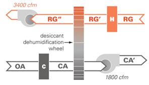
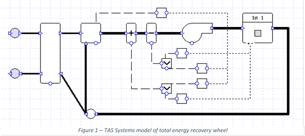
A passive total energy recovery wheel can be used to provide improved dehumidification. This preconditions the outside air and reduces the cooling capacity required by the coil. Latent and sensible heat are both removed from the outdoor air. This, in turn reduces the relative humidity of the zone whilst also saving on operating energy.
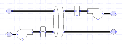
Below, figure 4 shows how the total energy recovery wheel is modelled in TAS systems with a normal heat exchanger.

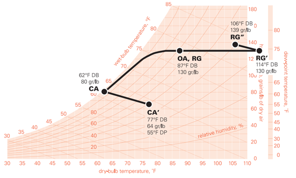
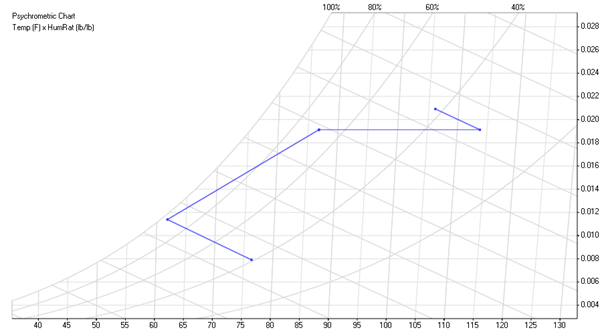
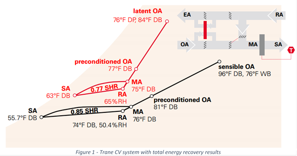
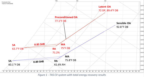
Figures 5 and 6 show the Trane and TAS results of the simulations carried out. Both show a marginal improvement in performance from the basic control volume system, however this still does not meet the ASHRAE requirement – a maximum relative humidity of 60%. Further dehumidification is not possible unless the mixed-air humidity ratio is reduced to less than the return air. This cannot be done without the implementation of another cooling coil. There is also a reduction in the energy required to cool the systems. This will be shown later.

Mixed Air Bypass

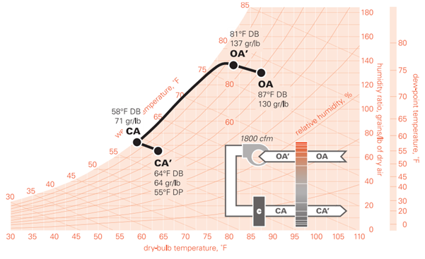
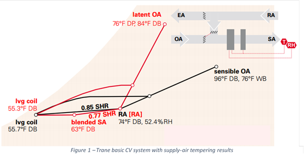
Mixed-air bypass utilizes dampers to increase indirect dehumidification for the constant volume air handler. This mixes cold, dry air leaving the cooling coil with warm, moist air that is a mixture of return air and outdoor air. This improves the performance of indirect dehumidification. There is a small trade off as more ducting is required, increasing the initial installed cost.
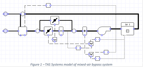
Below, figure 7 shows the TAS model of a mixed-air bypass system. This includes dampers to direct the flow of the air to bypass the cooling coil when a latent load exists, allowing increased dehumidification to be done on a smaller amount of air.

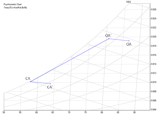
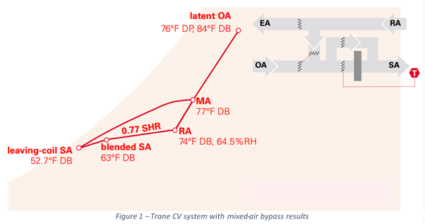
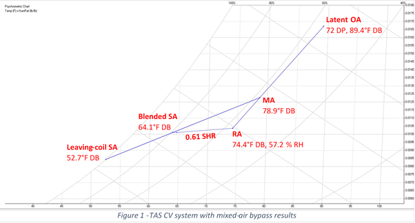
Figures 8 and 9 show the Psychrometric results for the mixed-air bypass system as found by Trane and TAS. In the case of this system, air will only bypass the cooling coil when there is a latent load present. For this reason the sensible load values can be found in figures 2 and 3 for the Trane and TAS examples respectively.
This system has the best performance results as seen so far. It is the first layout technique that, with the TAS climate and building, reduces the humidity to below the 60% ASHRAE established threshold. However, this is done under the peak latent load. All mixed air passes through the cooling coil under sensible load, meaning that no further dehumidification is done relative to the original basic CV example.

Seperate Paths

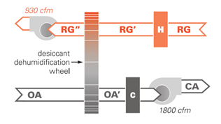
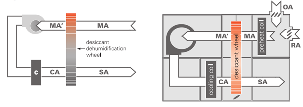
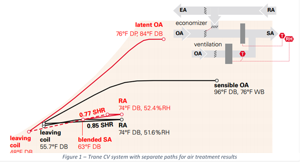
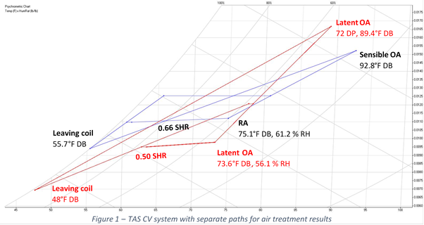
One form of direct dehumidification is the separate path technique. This involves treating the outside air and return air streams separately before mixing them. This separate treating can make more latent cooling removable occur that the previously discussed models.
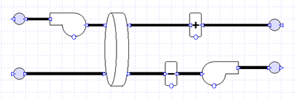
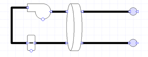
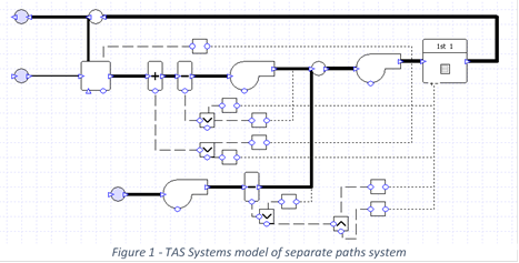
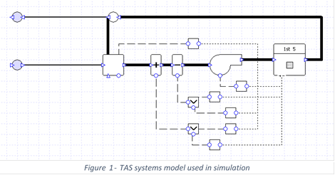
Below, figure 10 shows the TAS model of the separate path layout. The lower cooling coil is not only controlled by temperature, but also by relative humidity. This stream is then mixed with the return air stream that is used in the previous models.

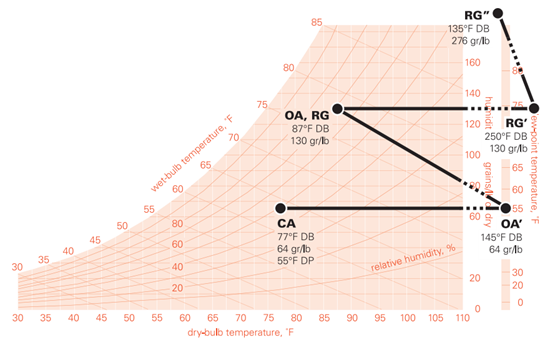
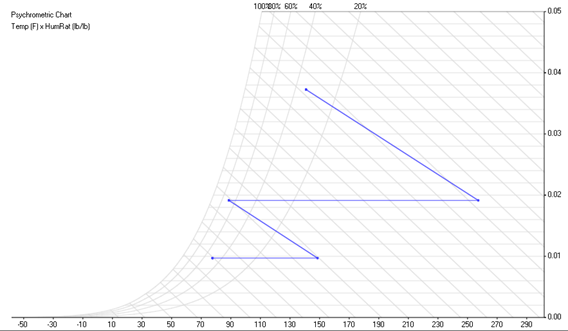
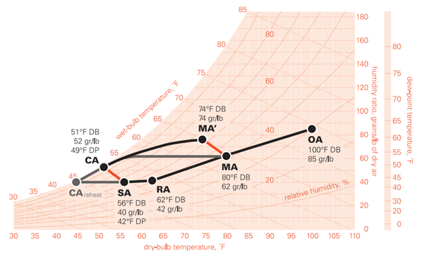
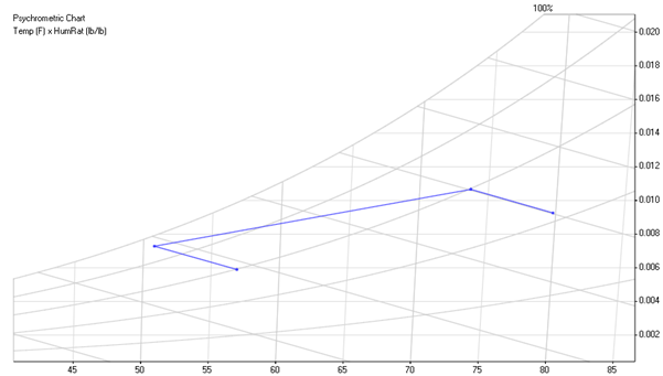
Figures 11 and 12 show the Psychrometric results for the separate air method. The performance between the Trane and the TAS models differ due to some limiting factors. In the TAS example the main point stopping the further dehumidification of the air is the leaving coil temperatures. These mean that the upon

Supply Air Tempering

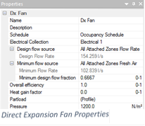
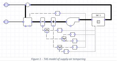
Supply-air tempering adopts the method of using a cooling coil directly followed by a heating device in series. This means that the cool is free to cool as much as is required to remove enough latent heat from the air. Directly after the coil, this air is often too cool to be placed directly into the zone so it is heated up to the desired temperature. The result is air at the desired temperature with a named relative humidity. The cooling coil is controlled not only by temperature, as has previously the case, but by a humidistat as well. Enough cooling is done to meet either the sensible load, or if a reduction in humidity is required, cooling to reduce the latent heat in the air.
Below, figure 13 shows TAS systems layout of the supply air tempering method. The only change between this and the original basic CV model is the use of a humidistat on the cooling coil. The heating coil then automatically reheats the air up to the required temperature to meet the zone temperature as set by the thermostat.

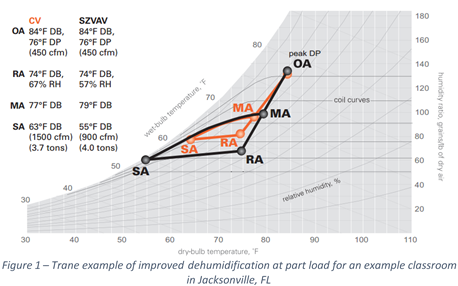
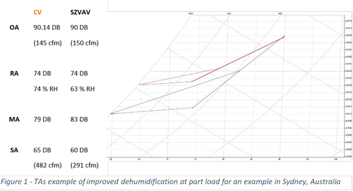
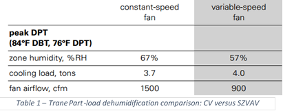
Figures 14 and 15 below show the Psychrometric results for the Trane and TAS systems simulations. As can be seen, supply-air tempering means that the relative humidity in the zone can always be controlled to the desired point. This is true for both peak sensible load and peak latent load. When designing the CV system, the size of the cooling coil needs to be sized to meet the loads both the sensible and design condition. This is automatically calculated in TAS systems.


The results show that both Trane and TAS expect a dramatic increase in dehumidification performance.

Comparison of Dehumidification Enhancements

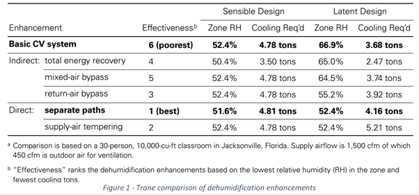
Below are comparisons of the dehumidification and cooling loads of the Trane and TAS simulations. Figure

Sensible Design Latent Design
Enhancement Effectiveness Zone RH Cooling Req. Zone RH Cooling Req.
Basic CV System 5 61.9% 0.92 tons 71.7% 0.7 tons
Total energy recovery 3 61.6% 0.77 tons 71.2% 0.58 tons
Mixed-air bypass 4 61.9% 0.92 tons 57.2% 1.06 tons
Seperate paths 2 60.2% 1.70 tons 56.1% 1.84 tons
Supply air tempering 1 52.0% 1.27 tons 52.0% 1.31 tons

Looking at the separate paths model in figure 17, more cooling is required at the latent load relative to the sensible load. In the Trane example this is not the case. This is due to the greater latent load present in the TAS climate model used. This is shown by the lower sensible heat ratio present when comparing figures 11 and 12. This means that more cooling has to be done to remove the heat. As well as this there is a greater specific load on the coil when at the latent condition. This is shown in the Psychrometric charts previously seen.
From the TAS simulations it can be seen that supply-air tempering is the best means of dehumidification. The best form will differ with varying climates that experience different sensible and latent loads.]]>

Use of Ice Storage in Building Design

Introduction

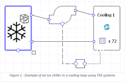
The purpose of this document is to demonstrate TAS systems’ ability in modelling ice storage systems with relation to the ‘Trane Engineer’s Newsletter Volume 36-3’. This is done by mimicking the examples of ice chillers in the newsletter to show that given results are achievable. TAS Systems has the ability to accurately implement ice storage of any size. TAS can show how energy consumption will differ and also how this will affect the running costs of the cooling system. This can not only be used as a prospective planning tool but also as a means of optimization, by showing how operating the cooling system differently could change the outcome.
Ice storage air conditioning creates ice by the means of a chiller. The ice can then be used at a later time for cooling. Ice can be made at night when electricity is in low demand and does not cost as much lowering the operating costs for the consumer. Ice storage can also mean that a smaller chiller is required. This is because the chiller can work more constantly, allowing the stored ice to be used at peak times when a smaller chiller would otherwise be unable to supply the required cooling. A smaller chiller would be desirable as it will reduce capital costs via any peak load tariffs that may be in effect where the system is based, as well as by reducing the initial purchase price of the chiller.

1.0 – Traditional Chiller

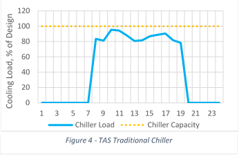
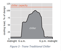
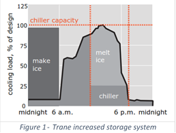
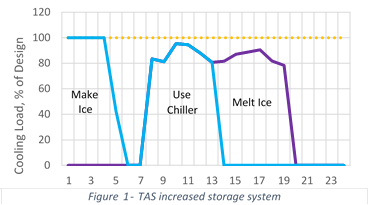
A traditional chiller needs to be sized so that it can always supply enough cooling to the building, even in the hottest days of the year. This leaves the system with an oversized chiller for the rest of the year. Figure 3 shows Trane’s representation of this and Figure 4 shows the results taken from a TAS Systems example. The data in the TAS example is taken from the hottest day of the year. This day decides how big the chiller needs to be sized. As in the Trane example, this size can be specified to be a factor of safety over the required size.

2.0 – Reducing Demand and Peak Consumption

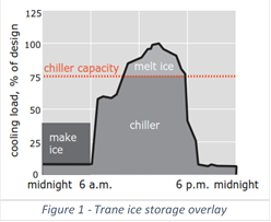
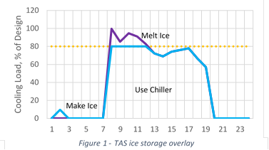
Figures 5 and 6 show how the size of a chiller can be reduced. The implementation of an ice storage chiller means that any required cooling above what the chiller has been sized for can done by the stored ice. This is shown by overlaying the area by which an ice chiller would reduce the peak consumption. A chiller sized at 80% of the original has been used.
Note that the TAS example (figure 6) only has a small load dedicated to making ice in the early hours of the day. This is because there is remaining ice from the previous day of the simulation, meaning that not much needed to be made to fill up the storage.
It is worth noting that when using this strategy, unless the climate is very constant, the ice storage will only be used for cooling in the hottest summer months. More money could be saved by implementing a more complex control strategy that used the stored ice for cooling when it is known that the chiller would not require supplementation when the stored ice runs out.

3.0 – Increased Storage System

By increasing the system storage size, much of the load can be shifted to the off peak hours where electricity is cheaper. This has the benefit of reducing the overall utilities charges for the system. Depending on how the system is managed this can also reduce the size of the chiller required further. In this case peak charges apply in the afternoon, so the ice that has been created overnight is used to cool the building in the afternoon, when otherwise the chiller would be required to work at a high operating cost.

4.0 – Cost Benefit of Ice Storage System

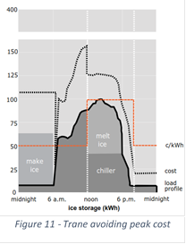
Operating a chiller during off peak hours will save money relative to on peak times. The following graphs show that without ice storage the chiller will be operating near its peak whilst the tariff is at the most expensive. In this case the engineering newsletter outlines that the maximum charge rate lies between 12pm and 6pm.


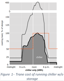
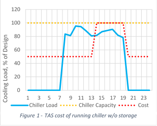
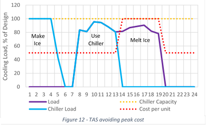
When ice storage has been implemented the chiller need not operate at high loads during times of peak charge. Figures 11 and 12 show how ice can be melted in peak times to avoid the high costs.

5.0 – Results of an Ice Storage Chiller Case Study

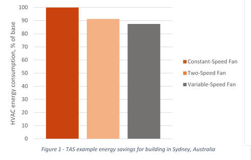
A small example of how an ice storage chiller could be implemented in TAS has been carried out. The building and location taken are in Sydney, Australia, with a fairly sizeable building consuming 7819 MMBtu/year.
It was assumed that peak consumption hours were in the afternoon, when cooling accounts for most of the energy usage in a Sydney office environment. It is at this time that the ice storage is used for cooling instead of employing the use of the chiller.
First a benchmark for the building was carried out with a chiller sized so that it would meet the cooling requirements throughout the year. Then the chiller was reduced in size by 20% meaning that ice storage rated at 2500 Ton-Hrs was implemented in order to meet the extra demand. The chiller size was then increased to the original size but with extra ice storage, 3000 Ton-Hrs. In table 1 it is shown that with each change, despite being an increase in energy consumption, there is significant cost savings.
Table 1 – Energy and cost analysis for differing chillers and storage capacity

Original Chiller (sized at 100%) 80% Chiller 2500 Ton-Hr 100% Chiller 3000 Ton-Hr
Energy (MMBtu/Year) Cost($) Energy (MMBtu/Year) Cost($) Energy (MMBtu/Year) Cost($)
7819 130876 7829 123193 7829 123166
Reduction ($) 7863 7710
% reduction -0.13 5.87 -0.13 5.89

This saving would also be much greater in countries such as America where there is also a charge for the peak demand usage in both peak and off peak hours. The demand charge is at a rate per kW. This charge would be significantly reduced with ice storage as the chiller will not be used to the same extent during the peak hours, meaning that the charge incurred by the company would be significantly less. An example of this is shown in table 2. From the Trane newsletter it stated that in peak times the demand is $12 per kW whilst off peak the demand is $5 per kW.
Table 2 – February example of peak demand energy cost savings

Original Chiller (sized at 100%) 80% Chiller 2500 Ton-Hr
Peak ($12 per kW) Off Peak ($5 per kW) Peak ($12 per kW) Off Peak ($5 per kW)
Peak Demand (kW) 839 60 481 436
Incurred Demand Cost ($) 10068 300 5772 2180
Total Demand Cost ($) 10368 7952

]]>

Cold Air Makes Good Sense

Introduction

The purpose of this document is to show the ability of TAS to measure HVAC performance with specific relation to the Trane engineering newsletter entitled ‘Cold Air Makes Good Sense’ Volume 29-2. The main principle to be reviewed is supplying air to a zone requiring cooling at a lower temperature than traditionally done. Supplying the air at a lower temperature means that less air needs to be supplied. This means that the supply air fan can be turned down. This reduction in supply air volume has many benefits including;
  • Smaller air-handling equipment
  • Smaller VAV terminals
  • Smaller Ductwork
  • Shorter floor to floor height (less space needed in between floors)
  • Less Fan horsepower
One effect of using colder supply air is the reduction in relative humidity in the cooled zones. This lower relative humidity deters the growth of mould and mildew and means that furnishings and carpets and other building materials are less inclined to developing moisture-related odours. Comfort can be improved when using cold air supply comes from increasing the room set point by a few degrees. The increased temperature means that lightly dressed people enjoy the warmer temperature, whilst heavier dressed people appreciate the lower relative humidity of the zone, so do not require the zone to be at the cooler temperature.

TAS Systems Model

A model was generated in TAS systems to be used in simulations for the traditional and cold supply air. The model made is a simple single zone VAV system with simulations run for both supply air criteria, allowing results to be collected and organised. Below, figure 1 shows this model as seen in TAS Systems.

Conditions Comparison

The cold air model differed from the traditional by lowering the supplied air from 55 Degrees Fahrenheit to 45. As well as this the upper operating condition for the room was increased from 76 to 79. The fan was left to be sized by the design conditions. The conditions and their outcomes are shown below in Tables 1 and 2.
Tas comparison of airside design
Conventional Cold Air
Supply Air (oF) 55 45
Room Set Point (oF) 72-76 72-79
Room Humidity Average Over 1 Year Simulation (%) 61.5 43.7
Cooling-Coil Δ T(oF) 20 33
Airflow Rate for Space Sensible Cooling Load (cfm/ton) 841 517
As can be seen in Table 2, the implementation of a cold air strategy results in a reduced airflow rate for space sensible cooling load of 39%. As a percentage reduction this is extremely close to the Trane example which finds a reduced airflow of 39%.

Impacts on System Design

The Trane engineering newsletter outlines how condensation is a major issue that many buildings encounter. It can lead to mould, as well as odour issues that can contribute to indoor air quality problems that can risk the occupant’s health. Cold air supply reduces the chance of condensation due to the lower relative humidity conditions that the zone will experience. Looking back to table 2, the average relative humidity in the zones during operating hour reduced from 61.5% to 43.7% in the TAS simulation. The lower humidity is attributed to the lower dew-point temperature of the air in the room, meaning that air has to be cooled more than air from a traditional system in order to induce condensate.

Supply Fan

The reductions in size of the supply fan have been quantified in tables 3 and 4. It can be seen that the reduction in maximum airflow is greater than that of the average airflow. The size of the fan is reduced by 44% in the TAS simulation, whereas in the Trane example it is reduced by 39%. This smaller required fan capacity means that a smaller fan can be used, saving on electricity costs as well as reducing the price of the initial purchase. Savings in power consumption are in line with the savings in airflow rate for space sensible cooling load, with both examples saving 39% again.
Tas comparison of supply fans
Air Temperature (oF) 55 45
Airflow Volume (cfm) 9844 5555
Total Static Pressure (wg) 3 3
Power Consumption (bhp) 9.29 5.24

Installed Power

Power usage must be compared in order to quantify what sort of financial savings a cold air supply strategy could be made. Tables 5 and 6 show the Trane and TAS comparisons of power savings. The results show similar savings with Trane expecting a 10% saving whilst TAS simulation also showed a 10% saving.
Tas comparison of installed power
Supply Air Temperature (oF) 55 45
Fans (kW) 6.49 3.46
Pumps (kW) 1.72 1.74
Cooling (kW) 42.95 40.85
Total Power Consumption (kW) 51.13 46.05
10% Saving
The difference in the proportional breakdown of installed power between the Trane and TAS results can be attributed to a few differences. The TAS simulation was done using an Australian climate model whilst Trane used an American location. This may be significant as the American location could have much higher ambient humidity levels relative to Australia. Also, although little is known about what data was used by Trane, it would be reasonable to assume that Australia is likely to be hotter, hence the larger cooling load proportionate to the installed system. The sizes of the systems used also differs, with Trane operating a whole building whilst, for simplicity of results, the TAS simulation only analyses a single room. TAS also looks at the results over a whole year of use whereas Trane appears to only sample one hour of operation. The TAS results have been averaged over the operating hours in a year to give results that are of a similar magnitude.